In this notebook, we will first learn how to transform NetworkX graphs into DeepSNAP representations. Then, we will dive deeper into how DeepSNAP stores and represents heterogeneous graphs as PyTorch Tensors.

Lastly, we will build our own heterogenous graph neural netowrk models using PyTorch Geometric and DeepSNAP. We will then apply our models for a node property prediction task; specifically, we will evaluate these models on the heterogeneous ACM node prediction dataset.

 DeepSNAP Basics

 在之前的 Colabs 中，我们分别使用了图形类（NetworkX）和图形张量（PyG）表示法。图类 nx.Graph 提供了丰富的分析和操作功能，例如聚类系数和 PageRank。要将图输入模型，我们需要将图转换为张量表示，包括边张量 edge_index、节点属性张量 x 和 y。但只使用张量（如 PyG 数据集和数据中的图格式）会降低许多图操作和分析的效率和难度。因此，在本 Colab 中，我们将使用 DeepSNAP，它结合了这两种表示法，并为 GNN 训练/验证/测试提供了完整的管道。

import networkx as nx
from networkx.algorithms.community import greedy_modularity_communities
import matplotlib.pyplot as plt
import copy

if 'IS_GRADESCOPE_ENV' not in os.environ:
  from pylab import show
  G = nx.karate_club_graph()
  community_map = {}
  for node in G.nodes(data=True):
    if node[1]["club"] == "Mr. Hi": #type(node)  tuple(元组)
      community_map[node[0]] = 0
    else:
      community_map[node[0]] = 1
  node_color = []
  color_map = {0: 0, 1: 1}
  node_color = [color_map[community_map[node]] for node in G.nodes()]
  pos = nx.spring_layout(G) #spring_layout:用Fruchterman-Reingold算法排列顶点
  plt.figure(figsize=(7, 7))
  nx.draw(G, pos=pos, cmap=plt.get_cmap('coolwarm'), node_color=node_color)
  show()

#如果用一句话概括，那tuple类型就是“只读”的list，因为它有list类型大部分方法和特性。
那你可能要问，为什么还要有tuple类型？原因就是正因为它的“只读”特性，
在操作速度和安全性上会比list更快更好。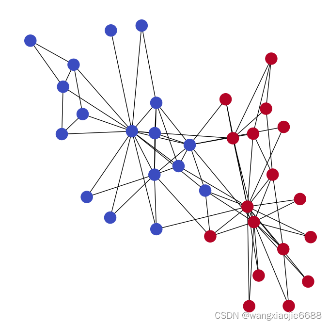

绘图代码，以后可以参考使用。

 Heterogeneous Graph Visualization

if 'IS_GRADESCOPE_ENV' not in os.environ:
  edge_color = {}
  for edge in G.edges():
    n1, n2 = edge
    edge_color[edge] = community_map[n1] if community_map[n1] == community_map[n2] else 2
    if community_map[n1] == community_map[n2] and community_map[n1] == 0:
      edge_color[edge] = 'blue'
    elif community_map[n1] == community_map[n2] and community_map[n1] == 1:
      edge_color[edge] = 'red'
    else:
      edge_color[edge] = 'green'

  G_orig = copy.deepcopy(G)
  nx.classes.function.set_edge_attributes(G, edge_color, name='color')
  colors = nx.get_edge_attributes(G,'color').values()
  labels = nx.get_node_attributes(G, 'node_type')
  plt.figure(figsize=(8, 8))
  nx.draw(G, pos=pos, cmap=plt.get_cmap('coolwarm'), node_color=node_color, edge_color=colors, labels=labels, font_color='white')
  show()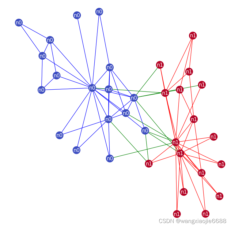

from deepsnap.dataset import GraphDataset

if 'IS_GRADESCOPE_ENV' not in os.environ:
  dataset = GraphDataset([hete], task='node')
  # Splitting the dataset
  dataset_train, dataset_val, dataset_test = dataset.split(transductive=True, split_ratio=[0.4, 0.3, 0.3])
  titles = ['Train', 'Validation', 'Test']

  for i, dataset in enumerate([dataset_train, dataset_val, dataset_test]):
    n0 = hete._convert_to_graph_index(dataset[0].node_label_index['n0'], 'n0').tolist()
    n1 = hete._convert_to_graph_index(dataset[0].node_label_index['n1'], 'n1').tolist()

    plt.figure(figsize=(7, 7))
    plt.title(titles[i])
    nx.draw(G_orig, pos=pos, node_color="grey", edge_color=colors, labels=labels, font_color='white')
    nx.draw_networkx_nodes(G_orig.subgraph(n0), pos=pos, node_color="blue")
    nx.draw_networkx_nodes(G_orig.subgraph(n1), pos=pos, node_color="red")
    show()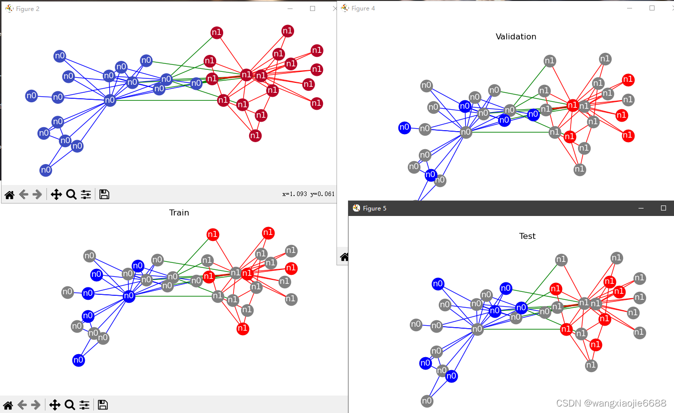

 

可视化。

 Heterogeneous Graph Node Property Prediction

First let's take a look at the general structure of a heterogeneous GNN layer by working through an example:

Let's assume we have a graph G, which contains two node types a and b, and three message types m1=(a,r1,a), m2=(a,r2,b) and m3=(a,r3,b). Note: during message passing we view each message as (src, relation, dst), where messages "flow" from src to dst node types. For example, during message passing, updating node type b relies on two different message types m2 and m3.

When applying message passing in heterogenous graphs, we seperately apply message passing over each message type. Therefore, for the graph G, a heterogeneous GNN layer contains three seperate Heterogeneous Message Passing layers (HeteroGNNConv in this Colab), where each HeteroGNNConv layer performs message passing and aggregation with respect to only one message type. Since a message type is viewed as (src, relation, dst) and messages "flow" from src to dst, each HeteroGNNConv layer only computes embeddings for the dst nodes of a given message type. For example, the HeteroGNNConv layer for message type m2 outputs updated embedding representations only for node's with type b.

NOTE: As reference, it may be helpful to additionally read through PyG's introduciton to heterogeneous graph representations and buidling heterogeneous GNN models: https://pytorch-geometric.readthedocs.io/en/latest/notes/heterogeneous.html

Creating Heterogeneous Graphs

First, we can create a data object of type torch_geometric.data.HeteroData, for which we define node feature tensors, edge index tensors and edge feature tensors individually for each type:

from torch_geometric.data import HeteroData

data = HeteroData()

data['paper'].x = ... # [num_papers, num_features_paper]
data['author'].x = ... # [num_authors, num_features_author]
data['institution'].x = ... # [num_institutions, num_features_institution]
data['field_of_study'].x = ... # [num_field, num_features_field]

data['paper', 'cites', 'paper'].edge_index = ... # [2, num_edges_cites] 这个2是啥意思？
data['author', 'writes', 'paper'].edge_index = ... # [2, num_edges_writes]
data['author', 'affiliated_with', 'institution'].edge_index = ... # [2, num_edges_affiliated]
data['paper', 'has_topic', 'field_of_study'].edge_index = ... # [2, num_edges_topic]

data['paper', 'cites', 'paper'].edge_attr = ... # [num_edges_cites, num_features_cites]
data['author', 'writes', 'paper'].edge_attr = ... # [num_edges_writes, num_features_writes]
data['author', 'affiliated_with', 'institution'].edge_attr = ... # [num_edges_affiliated, num_features_affiliated]
data['paper', 'has_topic', 'field_of_study'].edge_attr = ... # [num_edges_topic, num_features_topic]

这个2是啥意思？ 有些没搞懂。

The data object can be printed for verification.

HeteroData(
  paper={
    x=[736389, 128],
    y=[736389],
    train_mask=[736389],
    val_mask=[736389],
    test_mask=[736389]
  },
  author={ x=[1134649, 128] },
  institution={ x=[8740, 128] },
  field_of_study={ x=[59965, 128] },
  (author, affiliated_with, institution)={ edge_index=[2, 1043998] }, 
  (author, writes, paper)={ edge_index=[2, 7145660] },
  (paper, cites, paper)={ edge_index=[2, 5416271] },#这些数字怎么得来的？
  (paper, has_topic, field_of_study)={ edge_index=[2, 7505078] }
)

Automatically Converting GNN Models

Pytorch Geometric allows to automatically convert any PyG GNN model to a model for heterogeneous input graphs, using the built in functions torch_geometric.nn.to_hetero() or torch_geometric.nn.to_hetero_with_bases(). The following example shows how to apply it:

import torch_geometric.transforms as T
from torch_geometric.datasets import OGB_MAG
from torch_geometric.nn import SAGEConv, to_hetero


dataset = OGB_MAG(root='./data', preprocess='metapath2vec', transform=T.ToUndirected())
data = dataset[0] #这个要注意 咱也不知道为啥

class GNN(torch.nn.Module):
    def __init__(self, hidden_channels, out_channels):
        super().__init__()
        self.conv1 = SAGEConv((-1, -1), hidden_channels)
        self.conv2 = SAGEConv((-1, -1), out_channels)

    def forward(self, x, edge_index):
        x = self.conv1(x, edge_index).relu()
        x = self.conv2(x, edge_index)
        return x


model = GNN(hidden_channels=64, out_channels=dataset.num_classes)
model = to_hetero(model, data.metadata(), aggr='sum')
#用到的时候调试看参数细节吧 啥啊？

The process takes an existing GNN model and duplicates the message functions to work on each edge type individually, as detailed in the following figure.

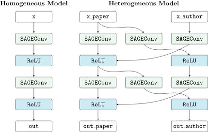
As a result, the model now expects dictionaries with node and edge types as keys as input arguments, rather than single tensors utilized in homogeneous graphs. Note that we pass in a tuple of in_channels to SAGEConv in order to allow for message passing in bipartite graphs.

Note：Since the number of input features and thus the size of tensors varies between different types, PyG can make use of lazy initialization （-1 啥需要参考代码学习？？？？）to initialize parameters in heterogeneous GNNs (as denoted by -1 as the in_channels argument). This allows us to avoid calculating and keeping track of all tensor sizes of the computation graph. Lazy initialization is supported for all existing PyG operators. We can initialize the model’s parameters by calling it once:

with torch.no_grad():  # Initialize lazy modules.
    out = model(data.x_dict, data.edge_index_dict)

from torch_geometric.nn import GATConv, Linear, to_hetero

class GAT(torch.nn.Module):
    def __init__(self, hidden_channels, out_channels):
        super().__init__() # -1 ???????????
        self.conv1 = GATConv((-1, -1), hidden_channels, add_self_loops=False)
        self.lin1 = Linear(-1, hidden_channels) #这里未涉及 dropout？？
        self.conv2 = GATConv((-1, -1), out_channels, add_self_loops=False)
        self.lin2 = Linear(-1, out_channels)

    def forward(self, x, edge_index):
        x = self.conv1(x, edge_index) + self.lin1(x)
        x = x.relu()  
        x = self.conv2(x, edge_index) + self.lin2(x)
        return x


model = GAT(hidden_channels=64, out_channels=dataset.num_classes)
model = to_hetero(model, data.metadata(), aggr='sum') #模型转换适用异构图/网络

def train():
    model.train()
    optimizer.zero_grad()
    out = model(data.x_dict, data.edge_index_dict)
    mask = data['paper'].train_mask
    loss = F.cross_entropy(out['paper'][mask], data['paper'].y[mask])
    loss.backward()
    optimizer.step()
    return float(loss)

Using the Heterogeneous Convolution Wrapper

The heterogeneous convolution wrapper torch_geometric.nn.conv.HeteroConv allows to define custom heterogeneous message and update functions to build arbitrary MP-GNNs for heterogeneous graphs from scratch. While the automatic converter to_hetero() uses the same operator for all edge types, the wrapper allows to define different operators for different edge types. Here, HeteroConv takes a dictionary of submodules as input, one for each edge type in the graph data. The following example shows how to apply it.

import torch_geometric.transforms as T
from torch_geometric.datasets import OGB_MAG
from torch_geometric.nn import HeteroConv, GCNConv, SAGEConv, GATConv, Linear


dataset = OGB_MAG(root='./data', preprocess='metapath2vec', transform=T.ToUndirected())
data = dataset[0]

class HeteroGNN(torch.nn.Module):
    def __init__(self, hidden_channels, out_channels, num_layers):
        super().__init__()

        self.convs = torch.nn.ModuleList()
        for _ in range(num_layers):
            conv = HeteroConv({
                ('paper', 'cites', 'paper'): GCNConv(-1, hidden_channels),
                ('author', 'writes', 'paper'): SAGEConv((-1, -1), hidden_channels),
                ('paper', 'rev_writes', 'author'): GATConv((-1, -1), hidden_channels),
            }, aggr='sum')
            self.convs.append(conv)

        self.lin = Linear(hidden_channels, out_channels)

    def forward(self, x_dict, edge_index_dict):
        for conv in self.convs:
            x_dict = conv(x_dict, edge_index_dict)
            x_dict = {key: x.relu() for key, x in x_dict.items()}
        return self.lin(x_dict['author'])

model = HeteroGNN(hidden_channels=64, out_channels=dataset.num_classes,
                  num_layers=2)

We can initialize the model by calling it once (see here for more details about lazy initialization)

with torch.no_grad():  # Initialize lazy modules.
     out = model(data.x_dict, data.edge_index_dict)

and run the standard training procedure as outlined here.

Heterogeneous Graph Samplers

import torch_geometric.transforms as T
from torch_geometric.datasets import OGB_MAG
from torch_geometric.loader import NeighborLoader

transform = T.ToUndirected()  # Add reverse edge types.
data = OGB_MAG(root='./data', preprocess='metapath2vec', transform=transform)[0]

train_loader = NeighborLoader(
    data,
    # Sample 15 neighbors for each node and each edge type for 2 iterations:
    num_neighbors=[15] * 2,
    # Use a batch size of 128 for sampling training nodes of type "paper":
    batch_size=128,
    input_nodes=('paper', data['paper'].train_mask),
)

batch = next(iter(train_loader)) #其他说明参照api说明吧

Heterogeneous Graph Learning — pytorch_geometric documentation (pytorch-geometric.readthedocs.io)

Training our heterogeneous GNN model in mini-batch mode is then similar to training it in full-batch mode, except that we now iterate over the mini-batches produced by train_loader and optimize model parameters based on individual mini-batches:

def train():
    model.train()

    total_examples = total_loss = 0
    for batch in train_loader:
        optimizer.zero_grad()
        batch = batch.to('cuda:0')
        batch_size = batch['paper'].batch_size
        out = model(batch.x_dict, batch.edge_index_dict)
        loss = F.cross_entropy(out['paper'][:batch_size],
                               batch['paper'].y[:batch_size])
        loss.backward()
        optimizer.step()

        total_examples += batch_size
        total_loss += float(loss) * batch_size

    return total_loss / total_examples
#具体训练细节有待调试研究 小批次训练，以抽样计算出的梯度估计整体梯度方向？

回到Colab5.2

 这里简单对比同构和异构的GraphSAGE更新规则：

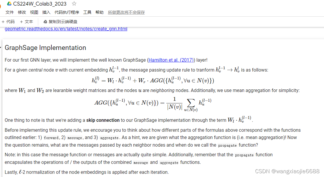
 异构图

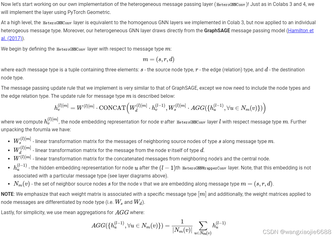
• W(l)[m]s - linear transformation matrix for the messages of neighboring source nodes of type s along message type m.
• W(l)[m]d - linear transformation matrix for the message from the node v itself of type d.
• W(l)[m] - linear transformation matrix for the concatenated messages from neighboring node's and the central node.
• h(l−1)u - the hidden embedding representation for node u after the (l−1)th HeteroGNNWrapperConv layer. Note, that this embedding is not associated with a particular message type (see layer diagrams above).
• Nm(v) - the set of neighbor source nodes s for the node v that we are embedding along message type m=(s,r,d).
• message type m

 代码解析见博文 cs224w_colab5.py 代码精读-CSDN博客